Introduction to TimescaleDB

Our world is full of various processes: tracking of goods delivery, currencies trading, monitoring of server resources, hotel bookings, selling goods or services etc. Since these processes occur over time, they can be described by time series data.

Successful businesses always take advantage of their data by analyzing it and then making predictions (e.g. predicting volume of sales for the next month) and business decisions (e.g. if the volume of sales grows then additional goods need to delivered to a warehouse).

There are a number of technologies for analysing the time series data. This article gives an introduction to one of them which is called TimescaleDB which is an open source solution for time series data analysis based on battle-tested PostgreSQL DBMS.

TL;DR

• Machines get smarter and produce lots of time series data.
• Time series data = timestamp + data describing a subject or a process at that corresponding point of time.
• TimescaleDB = PostgreSQL + timescaledb PostgreSQL extension.
• TimescaleDB provides much higher throughput than a vanilla PostgreSQL installation starting from approximately 100 million rows of data.
• There is a “docker flavor” of TimescaleDB so it can be relatively easy deployed into OpenShift.
• Use TimescaleDB if you love SQL and do not need true horizontal scalability (i.e. distribution of both data and computations).
• JPA + TimescaleDB = pain. Better use “SQL-native” tools.

Time series data

The amount of information, being processed and stored, grows rapidly as the world digitalizes. The digitalization (as well as the related term industry 4.0) is basically a fancy term for further and deeper automatization of processes in various sectors of economy (production, banking, transportation etc.). This automatization has been made possible by fact that machines and devices have got smarter and computationally more powerful (say “thanks” to the Moore’s law). They’ve also become interconnected with each other and with control systems and therefore they send tons of data which needs to be analysed and stored.

A big portion of this data is time series data. The time series data is data which describes how a subject or a process (e.g. position of a car, human pulse, cpu consumption of a server, currency exchange rate etc.) changes over time.

As a simple example consider a hypothetical person walking or running along the Mörsenbroicher Weg in Düsseldorf (from point A to point B):

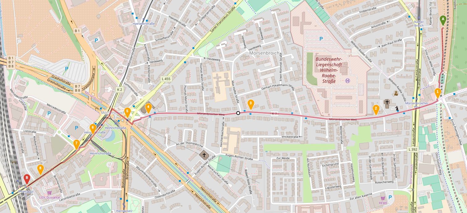
Suppose, the person’s phone is tracking his or her position and yields the following data which corresponds to the path above:

This data is time series data which describes the process of the person walking / running along the given path.

Time series data has the following typical properties:

• It has always a time dimension (it’s typically a timestamp).
• It is immutable i.e. append only data.
• It can arrive with variable frequency e.g. data can be collected daily or hourly and also at irregular intervals.
• It is often processed by window functions e.g. averaging values over hour intervals.
• It can often be viewed as a stream of events.

TimescaleDB

In short, TimescaleDB is PostgreSQL with installed timescaledb extension which adds some time series related “superpowers” to the DBMS. Therefore the tools from the PostgreSQL ecosystem also work with TimescaleDB e.g. backup tools (e.g. pg_dump), CLI and UI clients (e.g. psql and pgAdmin), visualisation tools (e.g. grafana), other PostgreSQL extensions (e.g. postgis) etc. and this is probably the main advantage and selling point of TimescaleDB. Additionally, you do not have to learn a new query language, just use the good old SQL together with a couple of functions from the timescaledb extension.

The central concept of the TimescaleDB is a hypertable. The hypertable is a virtual view consisting of many individual small tables holding the data which are called chunks. The chunks are created by partitioning the data by time interval and possibly some additional keys (e.g. GPS coordinates, temperature, location name, velocity etc.). This chunking technique gives the following benefits:

• Better query and insert rates thanks to adaptive chunking. The adaptive chunking means that chunk's intervals change depending on data volumes: more data – shorter intervals. It helps to keep chunks' sizes equal. The size of a chunk can be adjusted such that it, together with its indices, can fit entirely into memory which improves processing speed.
• Lower fragmentation: deletion of (old) data boils down to dropping entire chunks which is faster and avoids re-sizing of a table and its underlying files.

Since the hypertable is a view, you can do everything with it, what you normally do with a DB view: you can do selects, joins, filtering (via WHERE clause), ordering (via ORDER BY clause) etc. The fact that the hypertable is splitted into chunks does not complicate the way you interact with it.

In addition to usual SQL operations, inherited from PostgreSQL, TimescaleDB offers a couple of special functions for processing time series data e.g. time_bucket, first and last. time_bucket slices a time dimension into time intervals (buckets) of arbitrary duration. It does that by calculating the bucket’s start time for the time dimension and then one can GROUP BY the calulated time values. first and last aggregate functions select the first and the last written values of a column accordingly.

TimescaleDB markets itself as a relational DB suitable for processing time series data which scales vertically very well when the amount of data greatly increases. It claims to load one billion row database 15 times faster than a vanilla PostgreSQL installation and to provide throughput which is more than 20 times greater than that of the vanilla version.

Horizontal scaling is also possible via PostgreSQL replication mechanism but it is limited to data mirroring between instances. TimescaleDB cannot distribute computation out-of-the-box (i.e. execution of SQL queries). If a true horizontal scalability is desired, one must take care of the distribution of computation by himself (e.g. by implementing map-reduce atop of a cluster of TimescaleDB instances).

The following use cases are perfect for TimescaleDB:

• You are very happy with SQL and do not want to learn a new language for quering time series data. Additionally, you might already have relational data which you would like to combine with your time series data.
• You already use PostgreSQL for time series data analysis and are experiencing performance issues. You can relatively easy migrate to TimescaleDB (because it’s PostgreSQL under the hood) and thus process data faster. Additionally, you do not have the requirement that your system must have a true horizontal scalability (otherwise you would have considered stream processing systems such as combo Kafka + Flink or combo Kafka + Spark).

Actually, these 2 use cases can be condenced into the following decision tree:

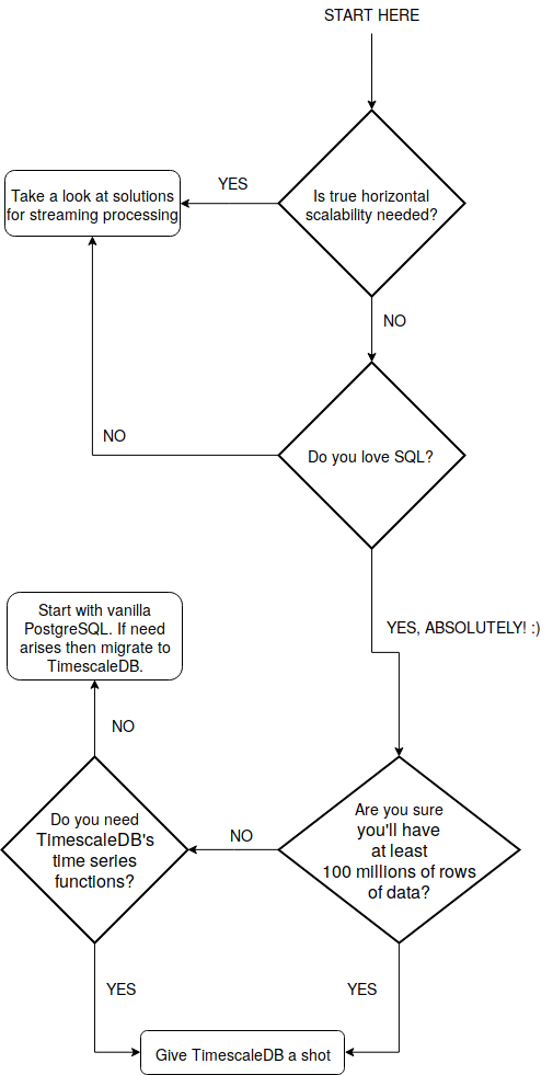
The “100 millions” (rows of data) number has been taken from the following graph:

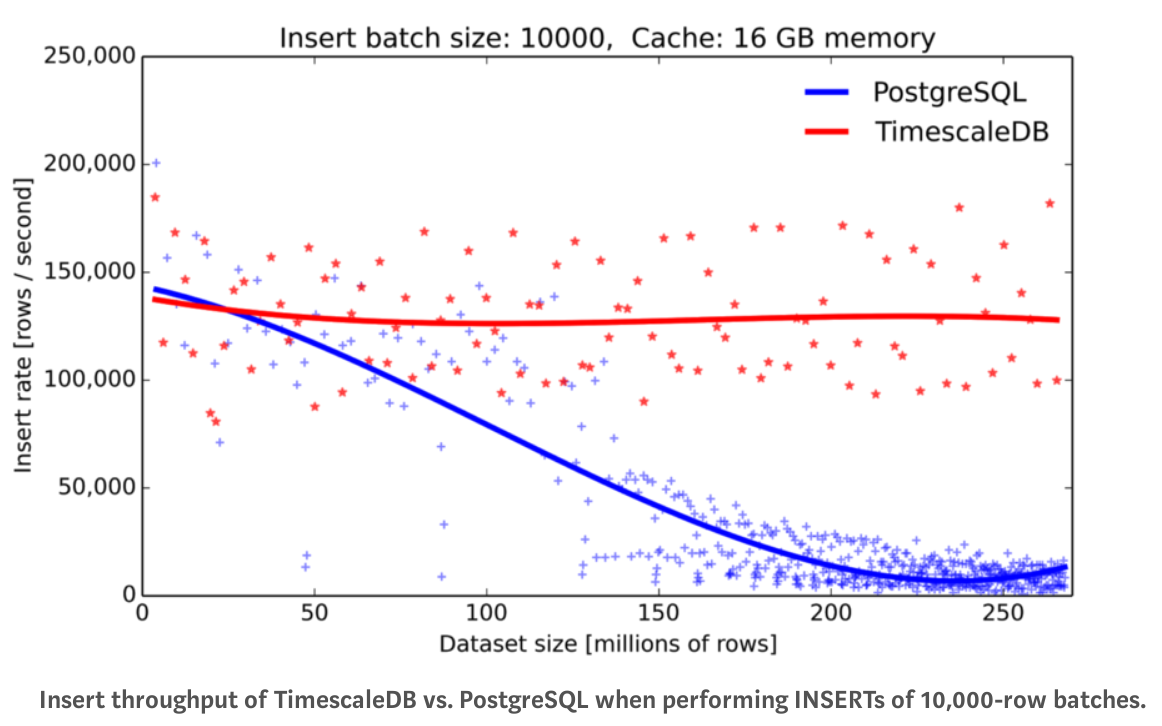
The original graph can be found here.

As you can see, at 100 millions of rows of data the insert rate of vanilla PostgreSQL is almost 2 times lower than of TimescaleDB. And the PostgreSQL’s insert rate continues to fall as the number of rows grows further.

Demo app

Idea

Consider a smartphone app collecting data from hypothetical persons. The data includes GPS location, height, person’s pulse, person’s body temperature and environment’s temperature. Since this data has time dimension (i.e. timestamp when it has been recorded), it’s time series data. The data needs to be saved and analysed. E.g. the average person’s pulse for every one minute interval needs to be calculated.

Solution plan

The mobile app is going to be imitated by a producer app. The producer will simulate data collected from a hypothetical person continuously walking or running along a closed route. This data is going to land in Kafka topic first and then it’ll be read by a consumer app which will write it into a TimescaleDB. Then the written time series data can be analysed using the TimescaleDB’s functions. Here is the overall app’s architecture:

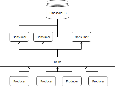
Kafka serves in this case as a buffer. E.g. in the case when consumers are down, the producers can continue working and send data. Of course one needs to make sure that the Kafka cluster is rock solid bacause if it is down then the data will be lost. Hopefully it can be achieved by increasing the number of Kafka brockers in the cluster and by tuning the replication factor for topics.

The demo OpenShift app can be found here. It can be built and deployed using the init.sh script:

git clone https://github.com/progaddict/timescale-demo.git
cd timescale-demo/utils
minishift start
# adjust the URL for your particular minishift's setup
oc login https://192.168.42.84:8443 -u admin -p admin
# admin user must have the cluster-admin role (required by strimzi)
. init.sh

Producer

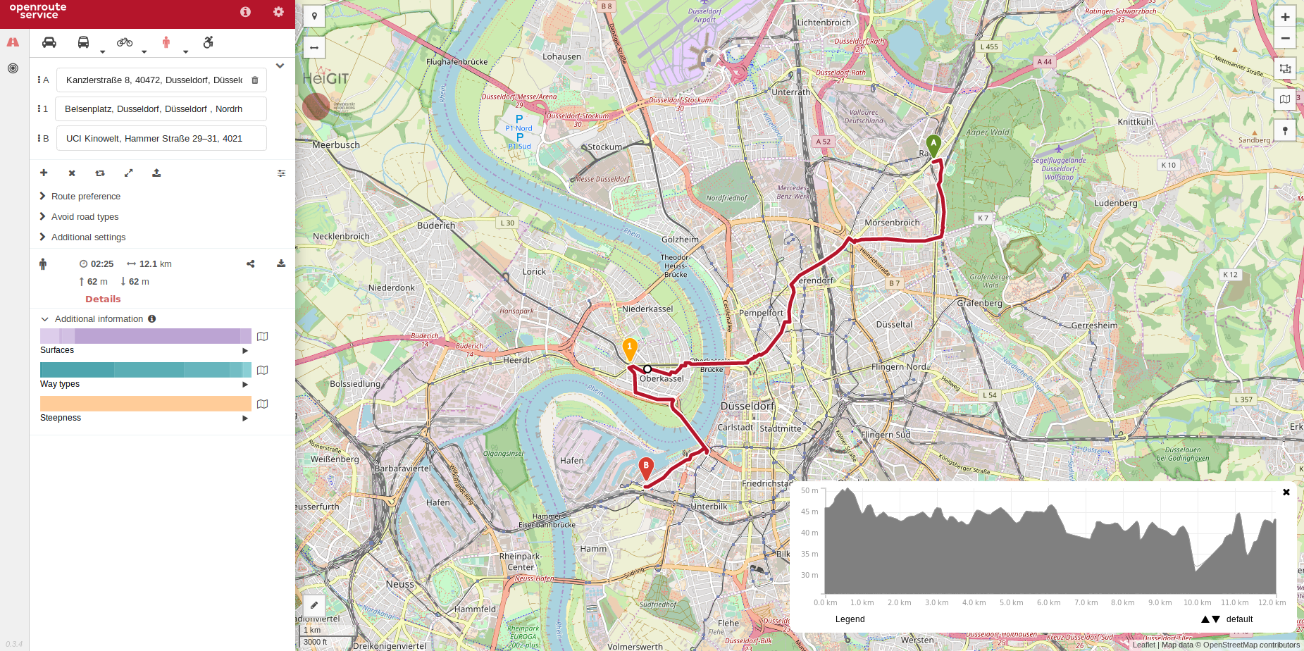
The producer simulates a person following a closed route consisting of two parts. The first part is the path from the ConSol Düsseldorf to the UCI Cinema (where JCon 2018 took place):

And the second part is the path leading back to the ConSol Düsseldorf (Kanzlerstraße 8):

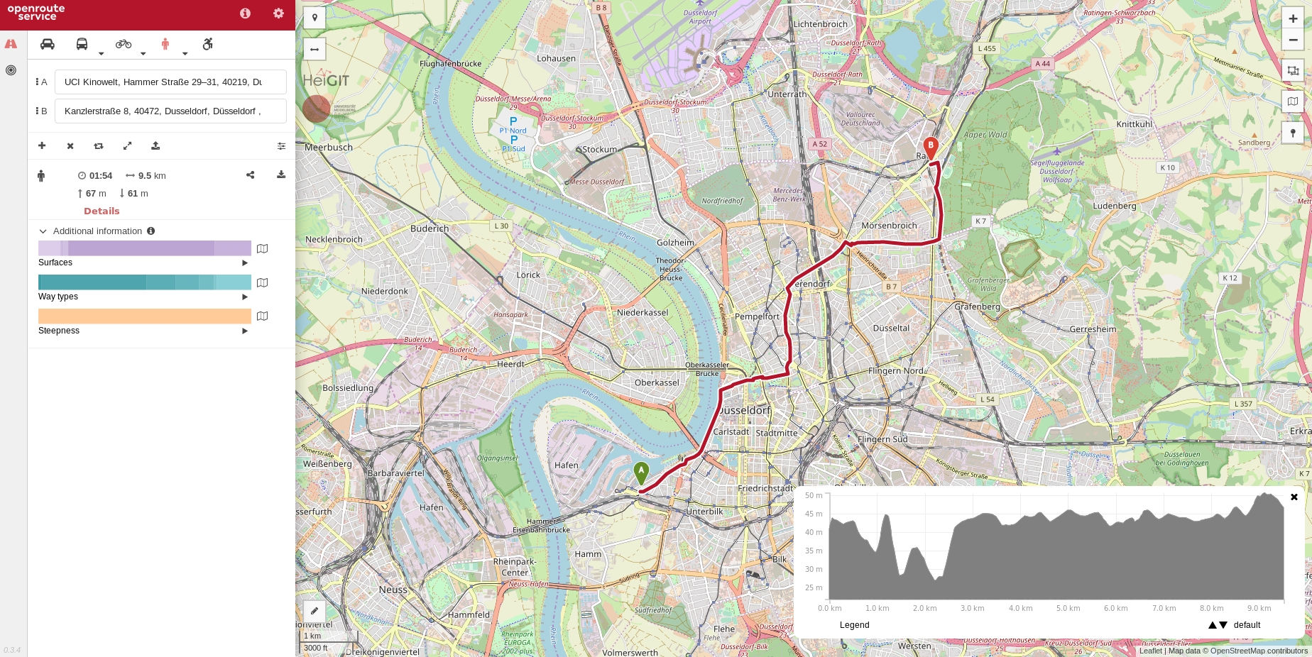
Thus the route is indeed a closed one: ConSol -> UCI Cinema -> ConSol. The route has been exported into *.geojson files (using the openroute service) containing its GPS and height information.

The producer generates the timeseries data the following way:

1. At the beginning the current person’s position is the first route’s point (i.e. GPS and height of the Kanzlerstraße 8 map point).
2. The person moves infinitely in the following loop:
   1. Producer app sleeps for a random time dt.
   2. Random velocity v is generated.
   3. Person’s new current GPS position and height are calculated via a simple interpolation from current GPS position and height in the direction of the next route point and its height, taking into account that he or she has advanced by v * dt distance units.
   4. Person’s pulse and body temperature are calculated as random values which depend on v.
   5. Environment’s temperature is also calculated as a random value (but it does not depend on v).
   6. The calculated values are sent into Kafka topic.

The implementation of this logic can be found here.

Kafka cluster

Demo app uses Strimzi which is basically a set of yaml files which can be used for deploying a Kafka cluster into OpenShift. Here is the part of the init.sh script which does that:

sed -i "s/namespace: .*/namespace: $OC_NAMESPACE/" \
    ${STRIMZI_INSTALL_DIR}/cluster-operator/*RoleBinding*.yaml

oc apply -n ${OC_NAMESPACE} -f ${STRIMZI_INSTALL_DIR}/cluster-operator

oc process -f ${STRIMZI_TEMPLATES_DIR}/cluster-operator/ephemeral-template.yaml \
    -p CLUSTER_NAME=${KAFKA_CLUSTER_NAME} \
    | oc create -n ${OC_NAMESPACE} -f -

The first command adjusts the namespace name in OpenShift’s role bindings for a Kafka cluster operator. The second command creates the cluster operator which is responsible for managing a Kafka cluster (an OpenShift’s resource of kind: Kafka) inside the OpenShift. The last command adds a Kafka cluster resource to an OpenShift cluster (which is then processed by the operator deployed a command earlier).

Consumer

Consumer is implemented as a Java EE app which periodically reads records from Kafka topic and writes them into DB. The implementation of the Kafka reader task can be found here. The task creates a Kafka reader for the specified topic:

private Optional<Consumer<Long, String>> createConsumer() {
    final Properties props = new Properties();
    props.put(ConsumerConfig.BOOTSTRAP_SERVERS_CONFIG,
            settings.getCommonKafkaSettings().getKafkaBootstrapServersConfig());
    props.put(ConsumerConfig.CLIENT_ID_CONFIG, settings.getCommonKafkaSettings().getKafkaClientIdConfig());
    props.put(ConsumerConfig.GROUP_ID_CONFIG, settings.getKafkaGroupIdConfig());
    props.put(ConsumerConfig.KEY_DESERIALIZER_CLASS_CONFIG, LongDeserializer.class.getName());
    props.put(ConsumerConfig.VALUE_DESERIALIZER_CLASS_CONFIG, StringDeserializer.class.getName());
    final Supplier<Consumer<Long, String>> supplier = () -> {
        final Consumer<Long, String> consumer = new KafkaConsumer<>(props);
        consumer.subscribe(settings.getCommonKafkaSettings().getKafkaTopics());
        return consumer;
    };
    return DurabilityUtils.getWithRetry(supplier, Duration.ofMinutes(1));
}

And then polls the messages in an infinite loop, deserializes them and persists the data into DB:

while (!closed.get()) {
    final ConsumerRecords<Long, String> records = consumer.poll(Duration.ofMillis(Long.MAX_VALUE));
    for (final ConsumerRecord<Long, String> record : records) {
        tryParseReceivedReadings(record.value()).ifPresent(dataManager::saveReadings);
    }
    consumer.commitSync();
}

DB

There is a “docker flavor” of TimescaleDB and therefore the DB can be deployed into OpenShift as a docker container instantiated from the following ImageStream:

apiVersion: v1
kind: ImageStream
metadata:
labels:
    app: timescale-demo
name: timescale-demo
spec:
lookupPolicy:
    local: false
tags:
- from:
    kind: DockerImage
    name: timescale/timescaledb:latest-pg10
    importPolicy: {}
    name: latest-pg10
    referencePolicy:
    type: Source

The docker image allows an initialization SQL script to be placed into /docker-entrypoint-initdb.d directory (which an be done via an OpenShift’s ConfigMap). The following SQL script initializes the app’s DB:

CREATE EXTENSION IF NOT EXISTS timescaledb CASCADE;

CREATE TABLE t_person (
    id          BIGINT            NOT NULL,
    first_name  VARCHAR(150)      NOT NULL,
    last_name   VARCHAR(150)      NOT NULL
);

ALTER TABLE t_person ADD CONSTRAINT t_person_pk PRIMARY KEY (id);

CREATE TABLE t_reading (
    person_id       BIGINT            NOT NULL,
    read_at         TIMESTAMPTZ       NOT NULL,
    device_id       UUID              NOT NULL,
    description     VARCHAR(150)      NOT NULL,
    value           NUMERIC(40,10)    NOT NULL,
    unit            VARCHAR(300)      NOT NULL
);

ALTER TABLE t_reading ADD CONSTRAINT t_reading_fk_person_id
    FOREIGN KEY (person_id) REFERENCES t_person (id) MATCH FULL;

SELECT create_hypertable('t_reading', 'read_at');

CREATE VIEW v_avg_pulse AS
    SELECT person_id, time_bucket('1 minutes', read_at) AS t, avg(value) as avg_pulse
    FROM t_reading
    WHERE description = 'pulse'
    GROUP BY person_id, t
    ORDER BY person_id, t DESC;

It creates tables for person’s data and time series data, generated by producers. It also creates a view v_avg_pulse which calculates average pulse of persons in 1 minute time intervals. This view is interfaced from the Java side via JPA as a table (in the consumer app):

@Entity
@Table(name = "v_avg_pulse")
@NamedQueries({ @NamedQuery(name = AvgPulse.Q_GET_FOR_PERSON,
        query = "SELECT ap FROM AvgPulse ap WHERE ap.personId = :personId") })
public class AvgPulse {

    public static final String Q_GET_FOR_PERSON = "Q_GET_FOR_PERSON";

    @Id
    @Column(name = "person_id", nullable = false)
    private Long personId;

    @Id
    @Column(name = "t", nullable = false)
    @Temporal(TemporalType.TIMESTAMP)
    private Instant time;

    @Column(name = "avg_pulse", nullable = false)
    private BigDecimal pulse;

    // setters and getters...
}

The time_bucket function takes the length of a desired time interval and the time dimension column, goes over the column and calculates the interval’s start time for each entry. It is intended to be used together with GROUP BY clause and aggregate functions. Consider as an example the following SQL query:

SELECT read_at                          AS t_actual,
    time_bucket('1 minutes', read_at)   AS t,
    value                               AS pulse
FROM t_reading
WHERE person_id = 1 AND description = 'pulse'
ORDER BY t_actual DESC;

Which yields results similar to these ones:

Now we can GROUP this data BY the t column and apply an aggregate function to the pulse column e.g. the avg function:

SELECT time_bucket('1 minutes', read_at)   AS t,
       avg(value)                          AS avg_pulse
FROM t_reading
WHERE person_id = 1 AND description = 'pulse'
GROUP BY t
ORDER BY t DESC;

And calculate the average pulse for each 1 minute interval for the person with id 1:

last and first TimescaleDB’s functions can also be used:

SELECT time_bucket('1 minutes', read_at)   AS t,
       first(value, read_at)               AS fisrt_recorded_pulse,
       last(value, read_at)                AS last_recored_pulse,
       avg(value)                          AS avg_pulse
FROM t_reading
WHERE person_id = 1 AND description = 'pulse'
GROUP BY t
ORDER BY t DESC;

Which yields the first and the last pulse recordings for each time interval in addition to the average pulse over the interval:

The view v_avg_pulse does the same average pulse calculation but does GROUP BY by both the time interval and person_id. The view is used to calculated average pulse measurements for a person with a given id when a request HTTP GET /reading/avg_pulse?personId=1 is processed (by the consumer app):

@Path("avg_pulse")
@GET
@Produces(MediaType.APPLICATION_JSON)
public List<AvgPulse> getAvgPulse(@QueryParam("personId") final Long personId) {
    if (personId == null) {
        return Collections.emptyList();
    }
    return dataManager.getAvgPulse(personId);
}

Here is an example response for person with id 1:

[
  {
    "personId": 1,
    "pulse": "90.1960424479958333",
    "time": "2018-10-27T18:43:00Z"
  },
  {
    "personId": 1,
    "pulse": "89.4347729407222222",
    "time": "2018-10-27T18:42:00Z"
  },
  {
    "personId": 1,
    "pulse": "89.3989980608970588",
    "time": "2018-10-27T18:41:00Z"
  },
  {
    "personId": 1,
    "pulse": "91.2908364937428571",
    "time": "2018-10-27T18:40:00Z"
  },
  {
    "personId": 1,
    "pulse": "88.9572873890111111",
    "time": "2018-10-27T17:23:00Z"
  },
  {
    "personId": 1,
    "pulse": "87.6238230550966667",
    "time": "2018-10-27T17:22:00Z"
  },
  {
    "personId": 1,
    "pulse": "86.4987895308696970",
    "time": "2018-10-27T17:21:00Z"
  },
  {
    "personId": 1,
    "pulse": "88.0265359836550000",
    "time": "2018-10-27T17:20:00Z"
  }
]

Difficulties along the way

One of the difficulties is consuming the TimescaleDB’s analytics from Java. Consider the following stored function:

CREATE OR REPLACE FUNCTION get_last_position(
    IN in_person_id BIGINT,
    OUT out_latitude NUMERIC(40,10),
    OUT out_longitude NUMERIC(40,10),
    OUT out_height NUMERIC(40,10)
)
AS $$
BEGIN
    SELECT last(value, read_at) INTO out_latitude
    FROM t_reading
    WHERE person_id = in_person_id AND description = 'latitude';
    SELECT last(value, read_at) INTO out_longitude
    FROM t_reading
    WHERE person_id = in_person_id AND description = 'longitude';
    SELECT last(value, read_at) INTO out_height
    FROM t_reading
    WHERE person_id = in_person_id AND description = 'height';
END;
$$ LANGUAGE plpgsql;

It calculates three output values depending on the given person_id. However, combo EclipseLink 2.7.3 + PostgreSQL JDBC 42.2.5 driver fails to interface with this stored function:

javax.persistence.PersistenceException:
    Exception [EclipseLink-7356] (Eclipse Persistence Services - 2.7.3.v20180807-4be1041): org.eclipse.persistence.exceptions.ValidationException
    Exception Description: Procedure: [get_last_position] cannot be executed because PostgreSQLPlatform does not currently support multiple out parameters

Probably some other combo JPA implementation + JDBC driver can do the job. However, it is pretty clear that “SQL-native” tools (i.e. tools from the PostgreSQL’s ecosystem) can consume TimescaleDB’s analytics much better.

Conclusion

TimescaleDB has currently only a handful of specialized functions for time series data analysis:

• first
• last
• time_bucket
• histogram

Nevertheless it is a promising solution for time series data analysis. The main selling point of TimescaleDB can probably be summarized into the following “motto”: use the power of the good old battle-tested SQL together with the PostgreSQL’s ecosystem. So if you love SQL, PostgreSQL and its ecosystem then you’ll find TimescaleDB easy and pleasant to use.

TimescaleDB is probably not a good fit for you if you need true horizontal scalability i.e. the ability to distribute both data and computations across a cluster of TimescaleDB instances. If you really need it then you should probably take a look at solutions for stream processing or, if you feel adventurous, implement e.g. map-reduce yourself in an ad-hoc way atop the TimescaleDB cluster.

TimescaleDB works best if used with “SQL-native” tools (i.e. the tools from the PostgreSQL’s ecosystem). It will probably be painful to weld JPA with TimescaleDB’s analytics.

P.S.

It is worth noting that TimescaleDB is not the only product which uses the idea of extending PostgreSQL with time series functionality. There is another very similar product: PipelineDB. However, the PipelineDB targets a slightly different use case:

PipelineDB should be used for analytics use cases that only require summary data, like realtime reporting dashboards.

It calculates analytics continuosly i.e. it does not save the arriving (i.e. being inserted) time series data but rather uses it to calculate new or update existing analytics and then throws the arrived data away.

Rerefences

• TimescaleDB’s architecture
• Motivation and design of TimescaleDB’s adaptive space/time chunking
• Docker flavor of TimescaleDB
• TimescaleDB tutorials
• TimescaleDB’s API
• Strimzi
• OpenShift